
One aspect of Excel that has always been a little cumbersome to me, and thus one I’ve avoided, are images. Up until very recently, Excel just didn’t handle images well at all. They were never really part of the data set, just a floating decoration above the data.
With the recent introduction of the IMAGE() function, that has all changed. It is now possible to insert an image as a proper cell data point that can be used by other functions as actual data. Instead of having a table showing warehouses and their contents printed, such as apples, oranges and bananas, you can now have a table showing the actual images of the apples, oranges and bananas. Or. you can have a shopping list that shows actual images of the items you are shopping for. For a business, maybe you use Excel for invoicing. Now you can add the logo of your business in strategic places on your invoice, or use images on the invoice line items. The IMAGE function is, in other words, a great way to break up the blocks of text and charts that Excel can be.
How to use the IMAGE function
Using the IMAGE function is simple. The syntax is as follows:
=IMAGE(“image_path”,[alt_text],[sizing],[height],[width])
The “image path” argument is the only required argument. You can specify a local file path, a URL or another cell that contains the path of the image, or URL. The function supports BMP, JPG/JPEG, GIF, TIFF, PNG, ICO, and also WEBP (WEBP is unsupported on Web and Android).
The optional arguments are:
[alt_text] – An optional argument that describes the image for accessibility purposes.
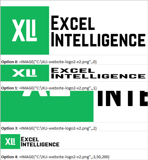
[sizing] – This argument specifies how Excel will handle the size of the image. “0” will fit the cell, “1” will fill the cell, “2” is the original size of the image, “3” is customer size.
- With the “0” option, the image will fit the cell the best it can while retaining its height and width proportions.
- The “1” option will fill the cell, squeezing and stretching the image to fill the cell with the image.
- The “2” option will show the image in its orginal size, regardless of the size of the cell, which means the image can be cut off if it’s larger than the cell.
- The “3” option allows you to set a custom height and width with the following arguments.
[height]: This argument specifies the height of the image in pixels for option “3” above, but is otherwise optional.
[width]: This argument specifies the width of the image in pixels for option “3” above, but is otherwise optional.
Here’s an example of how you might use the IMAGE function to insert an image into a cell:
=IMAGE("C:\XLI-website-logo2-v2.png",,3,50,200)
In this example, we’re inserting an image from a file located on the local file system. We’re setting the height to 50 pixels and width to 200 pixels. Below is screenshot from Excel that shows the same image shown using the four different sizing options.
If you prefer to use a image located on the web, simply replace the local file system path seen above with the URL.
One important thing to note is that the IMAGE function is only available in Excel for the web and in certain versions of Excel for Microsoft 365. If you’re using an older version of Excel, you may not have access to this function.
Tips for Using the Excel IMAGE Function
Now that we’ve explored how to use the IMAGE function, I’d like to share a few tips for using this function.
Choose the right image format: The Excel IMAGE function supports a variety of image formats, including JPEG, PNG, BMP, GIF, and TIFF. Make sure to choose the format that is best suited for your needs.
Choose the right image size: The IMAGE function allows you to specify the height and width of the image, but be careful not to make the image too large or it may become difficult to read. It’s usually best to keep images to a reasonable size, especially if you’re using them in a presentation. Also keep in mind that the size of the image correlates to the size of the image file itself. The same image in JPEG and PNG can have vastly different file sizes, which can impact performance, especially if the images are loaded from the Internet.
Use alt text to improve accessibility: Alt text is an important feature that can make your spreadsheet more accessible to users with visual impairments. Make sure to provide a short description of the image using the Excel “Alt Text” feature.
Use images sparingly: While images can be a powerful tool for improving the readability and engagement of your spreadsheet, it’s important not to overuse them. Use images sparingly and make sure that they are relevant to the content of your spreadsheet.